Statistiques Wireshark

Texte en anglais

1. Introduction

Wireshark provides a wide range of network statistics which can be accessed via the Statistics menu.

These statistics range from general information about the loaded capture file (like the number of captured packets), to statistics about specific protocols (e.g. statistics about the number of HTTP requests and responses captured).

• General statistics:

  • Summary about the capture file.
  • Protocol Hierarchy of the captured packets.
  • Conversations e.g. traffic between specific IP addresses.
  • Endpoints e.g. traffic to and from an IP addresses.
  • IO Graphs visualizing the number of packets (or similar) in time.

• Protocol specific statistics:

  • Service Response Time between request and response of some protocols.
  • Various other protocol specific statistics.

Note

The protocol specific statistics require detailed knowledge about the specific protocol. Unless you are familiar with that protocol, statistics about it will be pretty hard to understand.

2. The “Summary” window

General statistics about the current capture file.

Figure 8.1. The “Summary” window

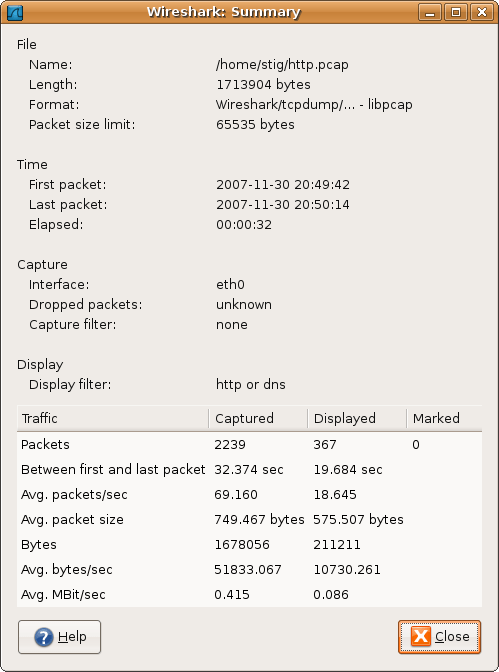
• File: general information about the capture file.
• Time: the timestamps when the first and the last packet were captured (and the time between them).
• Capture: information from the time when the capture was done (only available if the packet data was captured from the network and not loaded from a file).
• Display: some display related information.
• Traffic: some statistics of the network traffic seen. If a display filter is set, you will see values in the Captured column, and if any packages are marked, you will see values in the Marked column. The values in the Captured column will remain the same as before, while the values in the Displayed column will reflect the values corresponding to the packets shown in the display. The values in the Marked column will reflect the values corresponding to the marked packages.

3. The “Protocol Hierarchy” window

The protocol hierarchy of the captured packets.

Figure 8.2. The “Protocol Hierarchy” window

This is a tree of all the protocols in the capture. Each row contains the statistical values of one protocol. Two of the columns (Percent Packets and Percent Bytes) serve double duty as bar graphs. If a display filter is set it will be shown at the bottom.

The Copy button will let you copy the window contents as CSV or YAML.

Protocol hierarchy columns

Protocol This protocol’s name

Percent Packets The percentage of protocol packets relative to all packets in the capture

Packets The total number of packets of this protocol

Percent Bytes The percentage of protocol bytes relative to the total bytes in the capture

Bytes The total number of bytes of this protocol

Bits/s The bandwidth of this protocol relative to the capture time

End Packets The absolute number of packets of this protocol where it was the highest protocol in the stack (last dissected)

End Bytes The absolute number of bytes of this protocol where it was the highest protocol in the stack (last dissected)

End Bits/s The bandwidth of this protocol relative to the capture time where was the highest protocol in the stack (last dissected)

Packets usually contain multiple protocols. As a result more than one protocol will be counted for each packet. Example: In the screenshot IP has 99.9% and TCP 98.5% (which is together much more than 100%).

Protocol layers can consist of packets that won’t contain any higher layer protocol, so the sum of all higher layer packets may not sum up to the protocols packet count. Example: In the screenshot TCP has 98.5% but the sum of the subprotocols (SSL, HTTP, etc) is much less. This can be caused by continuation frames, TCP protocol overhead, and other undissected data.

A single packet can contain the same protocol more than once. In this case, the protocol is counted more than once. For example ICMP replies and many tunneling protocols will carry more than one IP header.

4. Conversations

A network conversation is the traffic between two specific endpoints. For example, an IP conversation is all the traffic between two IP addresses. The description of the known endpoint types can be found in Section 8.5, “Endpoints”.

4.1. The “Conversations” window

The conversations window is similar to the endpoint Window. See Section 8.5.1, “The “Endpoints” window” for a description of their common features. Along with addresses, packet counters, and byte counters the conversation window adds four columns: the start time of the conversation (“Rel Start”) or (“Abs Start”), the duration of the conversation in seconds, and the average bits (not bytes) per second in each direction. A timeline graph is also drawn across the “Rel Start” / “Abs Start” and “Duration” columns.

Figure 8.3. The “Conversations” window

Each row in the list shows the statistical values for exactly one conversation.

Name resolution will be done if selected in the window and if it is active for the specific protocol layer (MAC layer for the selected Ethernet endpoints page). Limit to display filter will only show conversations matching the current display filter. Absolute start time switches the start time column between relative (“Rel Start”) and absolute (“Abs Start”) times. Relative start times match the “Seconds Since Beginning of Capture” time display format in the packet list and absolute start times match the “Time of Day” display format.

The Copy button will copy the list values to the clipboard in CSV (Comma Separated Values) or YAML format. The Follow Stream… button will show the stream contents as described in Figure 7.1, “The “Follow TCP Stream” dialog box” dialog. The Graph… button will show a graph as described in Section 8.6, “The “IO Graphs” window”.

Conversation Types lets you choose which traffic type tabs are shown. See Section 8.5, “Endpoints” for a list of endpoint types. The enabled types are saved in your profile settings.

Tip

This window will be updated frequently so it will be useful even if you open it before (or while) you are doing a live capture.

5. Endpoints

A network endpoint is the logical endpoint of separate protocol traffic of a specific protocol layer. The endpoint statistics of Wireshark will take the following endpoints into account:

Tip

If you are looking for a feature other network tools call a hostlist, here is the right place to look. The list of Ethernet or IP endpoints is usually what you’re looking for.

Endpoint and Conversation types

Bluetooth A MAC-48 address similar to Ethernet.

Ethernet Identical to the Ethernet device’s MAC-48 identifier.

Fibre Channel A MAC-48 address similar to Ethernet.

IEEE 802.11 A MAC-48 address similar to Ethernet.

FDDI Identical to the FDDI MAC-48 address.

IPv4 Identical to the 32-bit IPv4 address.

IPv6 Identical to the 128-bit IPv6 address.

IPX A concatenation of a 32 bit network number and 48 bit node address, by default the Ethernet interface’s MAC-48 address.

JXTA A 160 bit SHA-1 URN.

NCP Similar to IPX.

RSVP A combination of varios RSVP session attributes and IPv4 addresses.

SCTP A combination of the host IP addresses (plural) and the SCTP port used. So different SCTP ports on the same IP address are different SCTP endpoints, but the same SCTP port on different IP addresses of the same host are still the same endpoint.

TCP A combination of the IP address and the TCP port used. Different TCP ports on the same IP address are different TCP endpoints.

Token Ring Identical to the Token Ring MAC-48 address.

UDP A combination of the IP address and the UDP port used, so different UDP ports on the same IP address are different UDP endpoints.

USB Identical to the 7-bit USB address.

Broadcast and multicast endpoints

Broadcast and multicast traffic will be shown separately as additional endpoints. Of course, as these aren’t physical endpoints the real traffic will be received by some or all of the listed unicast endpoints.

5.1. The “Endpoints” window

This window shows statistics about the endpoints captured.

Figure 8.4. The “Endpoints” window

For each supported protocol, a tab is shown in this window. Each tab label shows the number of endpoints captured (e.g. the tab label “Ethernet · 4” tells you that four ethernet endpoints have been captured). If no endpoints of a specific protocol were captured, the tab label will be greyed out (although the related page can still be selected).

Each row in the list shows the statistical values for exactly one endpoint.

Name resolution will be done if selected in the window and if it is active for the specific protocol layer (MAC layer for the selected Ethernet endpoints page). Limit to display filter will only show conversations matching the current display filter. Note that in this example we have GeoIP configured which gives us extra geographic columns. See Section 10.10, “GeoIP Database Paths” for more information.

The Copy button will copy the list values to the clipboard in CSV (Comma Separated Values) or YAML format. The Map button will show the endpoints mapped in your web browser.

Endpoint Types lets you choose which traffic type tabs are shown. See Section 8.5, “Endpoints” above for a list of endpoint types. The enabled types are saved in your profile settings.

Tip

This window will be updated frequently, so it will be useful even if you open it before (or while) you are doing a live capture.

6. The “IO Graphs” window

User configurable graph of the captured network packets.

You can define up to five differently colored graphs.

Figure 8.5. The “IO Graphs” window

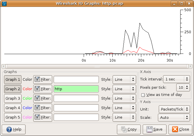
The user can configure the following things:

• Graphs

  • Graph 1-5: enable the specific graph 1-5 (only graph 1 is enabled by default)
  • Color: the color of the graph (cannot be changed)
  • Filter: a display filter for this graph (only the packets that pass this filter will be taken into account for this graph)
  • Style: the style of the graph (Line/Impulse/FBar/Dot)

• X Axis

  • Tick interval: an interval in x direction lasts (10/1 minutes or 10/1/0.1/0.01/0.001 seconds)
  • Pixels per tick: use 10/5/2/1 pixels per tick interval
  • View as time of day: option to view x direction labels as time of day instead of seconds or minutes since beginning of capture

• Y Axis

  • Unit: the unit for the y direction (Packets/Tick, Bytes/Tick, Bits/Tick, Advanced…) [XXX - describe the Advanced feature.]
  • Scale: the scale for the y unit (Logarithmic,Auto,10,20,50,100,200,500,…)

The Save button will save the currently displayed portion of the graph as one of various file formats.

The Copy button will copy values from selected graphs to the clipboard in CSV (Comma Separated Values) format.

Tip

Click in the graph to select the first package in the selected interval.

7. Service Response Time

The service response time is the time between a request and the corresponding response. This information is available for many protocols.

Service response time statistics are currently available for the following protocols:

• DCE-RPC
• Fibre Channel
• H.225 RAS
• LDAP
• LTE MAC
• MGCP
• ONC-RPC
• SMB

As an example, the DCE-RPC service response time is described in more detail.

Note

The other Service Response Time windows will work the same way (or only slightly different) compared to the following description.

7.1. The “Service Response Time DCE-RPC” window

The service response time of DCE-RPC is the time between the request and the corresponding response.

First of all, you have to select the DCE-RPC interface:

Figure 8.6. The “Compute DCE-RPC statistics” window

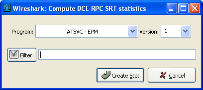
You can optionally set a display filter, to reduce the amount of packets.

Figure 8.7. The “DCE-RPC Statistic for …” window

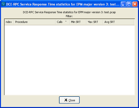
Each row corresponds to a method of the interface selected (so the EPM interface in version 3 has 7 methods). For each method the number of calls, and the statistics of the SRT time is calculated.

8. Compare two capture files

Compare two capture files.

This feature works best when you have merged two capture files chronologically, one from each side of a client/server connection.

The merged capture data is checked for missing packets. If a matching connection is found it is checked for:

• IP header checksums
• Excessive delay (defined by the “Time variance” setting)
• Packet order

Figure 8.8. The “Compare” window

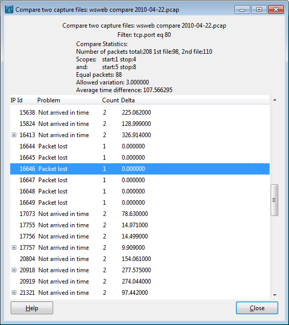
You can configure the following:

• Start compare: Start comparing when this many IP IDs are matched. A zero value starts comparing immediately.
• Stop compare: Stop comparing when we can no longer match this many IP IDs. Zero always compares.
• Endpoint distinction: Use MAC addresses or IP time-to-live values to determine connection endpoints.
• Check order: Check for the same IP ID in the previous packet at each end.
• Time variance: Trigger an error if the packet arrives this many milliseconds after the average delay.
• Filter: Limit comparison to packets that match this display filter.

The info column contains new numbering so the same packets are parallel.

The color filtering differentiate the two files from each other. A “zebra” effect is create if the Info column is sorted.

Tip

If you click on an item in the error list its corresponding packet will be selected in the main window.

9. WLAN Traffic Statistics

Statistics of the captured WLAN traffic. This window will summarize the wireless network traffic found in the capture. Probe requests will be merged into an existing network if the SSID matches.

Figure 8.9. The “WLAN Traffic Statistics” window

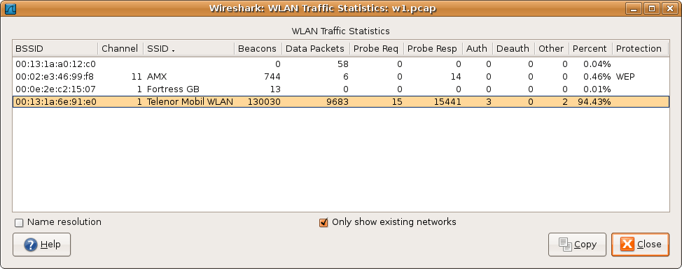
Each row in the list shows the statistical values for exactly one wireless network.

Name resolution will be done if selected in the window and if it is active for the MAC layer.

Only show existing networks will exclude probe requests with a SSID not matching any network from the list.

The Copy button will copy the list values to the clipboard in CSV (Comma Separated Values) format.

Tip

This window will be updated frequently, so it will be useful, even if you open it before (or while) you are doing a live capture.

10. The protocol specific statistics windows

The protocol specific statistics windows display detailed information of specific protocols and might be described in a later version of this document.

Some of these statistics are described at https://wiki.wireshark.org/Statistics.

Sources

• https://www.wireshark.org/docs/wsug_html/#ChStatistics